---
layout: post
title: Adjusting default hues of Landsat terralook images [part 1]
tags: [R,oce,satellites,landsat]
category: R
year: 2016
month: 02
day: 20
summary: The present scheme displays the land with on overly green tinge.
---

# Introduction

I posted an oce issue recently [1] that indicated my displeasure with the
present defaults for the hues of Landsat plots that use `band="terralook"`.
Others have reported similar problems, and this was enough to motivate some
experimentation.

I choose a region with which I am very familiar, namely the city in which I
live, Halifax Nova Scotia. I happen to have two Landsat scenes on my computer,
one from summer and one from winter, so I used them for my tests.

Readers who are unfamiliar with Halifax might want to consult a map to
understand place names in the following discussion of my reference points in
the Landsat images.

First, note that the chosen region contains a fair bit of ocean, but I lack
ground-truth on its colour, so I have no way to know if the hue on a given day
should be blueish, greenish, or grayish.

The scene also does not contain much in the way of red reference material, nor
yellow. I suppose other Landsat images show fields or deserts that would be
good for such colours, and I will on other people working on such domains to
let me know whether `plot.landsat` will need further adjustment for those hues.

In my reference images, I have three main elements: green areas, snow-covered
areas, which should have a light and neutral hue, and asphalt-covered areas
that should be dark and neutral.

Year-round, the region of Point Pleasant Park should be a green hue, because
the trees there are mostly coniferous. In the rest of the city, trees are
mostly deciduous, and so comparing summer and winter images will be helpful
there. The southern dockyard region and the train-tracks leading to it are
either covered by asphalt or gravel, and so should be neutral in tone.

# Procedure

The first step in the code is to create local files. This saves time, because
reading raw Landsat files is time consuming. (Note that the files are checked
into the git repository holding this blog, so that savvy readers can reproduce
the other steps of this posting without downloading 2Gb worth of Landsat
files.)

```{r eval=FALSE}
library(oce)
## 1. Create local-view datasets
Hc <- c(-63.57, 44.63)                 # south end of Halifax, NS
Hd <- 0.025 * c(1/cos(pi*Hc[2]/180), 1) # approx 5 km box
band <- c("red", "green", "nir") # lets us plot 'terralook'
## Wintertime
if (0==length(list.files(pattern="^Hw.rda$"))) {
    w <- read.landsat("/data/archive/landsat/LC80080292014065LGN00", band=band)
    Hw <- landsatTrim(w, ll=Hc-Hd, ur=Hc+Hd)
    save(Hw, file="Hw.rda")
    rm(w)
} else {
    load("Hw.rda")
}

## Summertime
if (0==length(list.files(pattern="^Hs.rda$"))) {
    s <- read.landsat("/data/archive/landsat/LC80070292014170LGN00", band=band)
    Hs <- landsatTrim(s, ll=Hc-Hd, ur=Hc+Hd)
    save(Hs, file="Hs.rda")
    rm(s)
} else {
    load("Hs.rda")
}
```

At this stage, we have `landsat-class` objects named `Hw` and `Hs` to work
with. It is convenient to set up a `demo` function that will plot a four-panel
plot.
```{r eval=FALSE}
demo <- function(red.f, green.f, blue.f, name="")
{
    if (!missing(name)) png(name, unit="in", width=6, height=3.1, res=150)
    par(mfrow=c(1,2))
    mar <- c(0.25, 0.25, 1, 0.25)
    mar <- c(2, 2, 1.5, 0.5)
    axes <- TRUE
    cex <- 0.8
    plot(Hw, band='terralook', red.f=red.f, green.f=green.f, blue.f=blue.f,
         mar=mar, axes=axes, cex=cex)
    mtext(sprintf("red.f=%g, green.f=%g, blue.f=%g", red.f, green.f, blue.f),
          side=3, line=0, adj=0, cex=cex)
    mtext(format(Hw[['time']], "%B %Y"), side=3, line=0, adj=1, cex=cex)
    plot(Hs, band='terralook', red.f=red.f, green.f=green.f, blue.f=blue.f,
         mar=mar, axes=axes, cex=cex)
    mtext(sprintf("red.f=%g, green.f=%g, blue.f=%g", red.f, green.f, blue.f),
          side=3, line=0, adj=0, cex=cex)
    mtext(format(Hs[['time']], "%B %Y"), side=3, line=0, adj=1, cex=cex)
    if (!missing(name)) dev.off()
}
```

Now, we can try some tests. Leaving out `name` argument will produce
interactive plots, and indeed that is how I selected the values I show below.
Note that I have hard-coded the plot sizes, rather than use Jekyll and
Rmarkdown to do that.

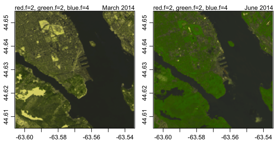
**Case 1.**

Present-day default, much too green overall. Look especially at the
snow-covered citadel/commons region near 63.58W and 44.65N.

```{r eval=FALSE}
demo(2, 2, 4, "2016-02-20-landsat-1.png")
```
![center](https://dankelley.github.io/figs/2016-02-20-landsat-1.png) 

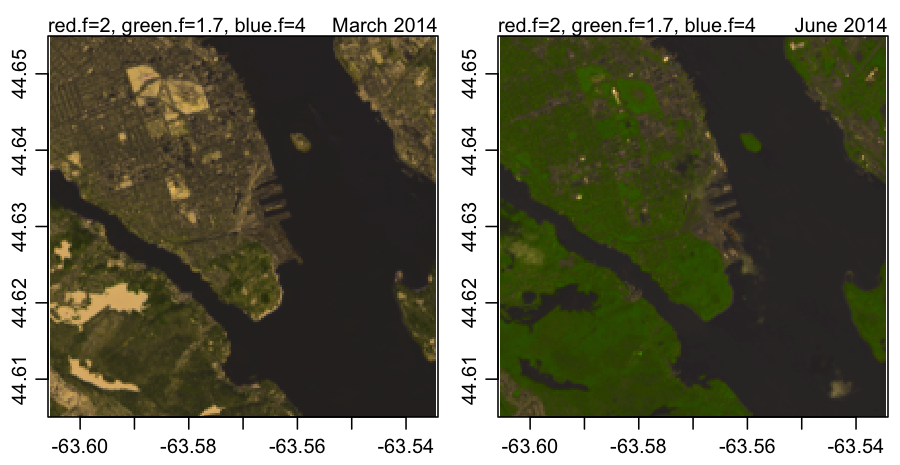
**Case 2.**

The greens are more reasonable now, e.g. still green in the evergreen trees of
Point Pleasant Park, and along the railway cut line that crosses the city a
little south of 44.63N. However, there a slight yellow-reddish hue overall (see
especially the snow-covered citadel).

```{r eval=FALSE}
demo(2, 1.7, 4, "2016-02-20-landsat-2.png")
```
![center](https://dankelley.github.io/figs/2016-02-20-landsat-2.png) 

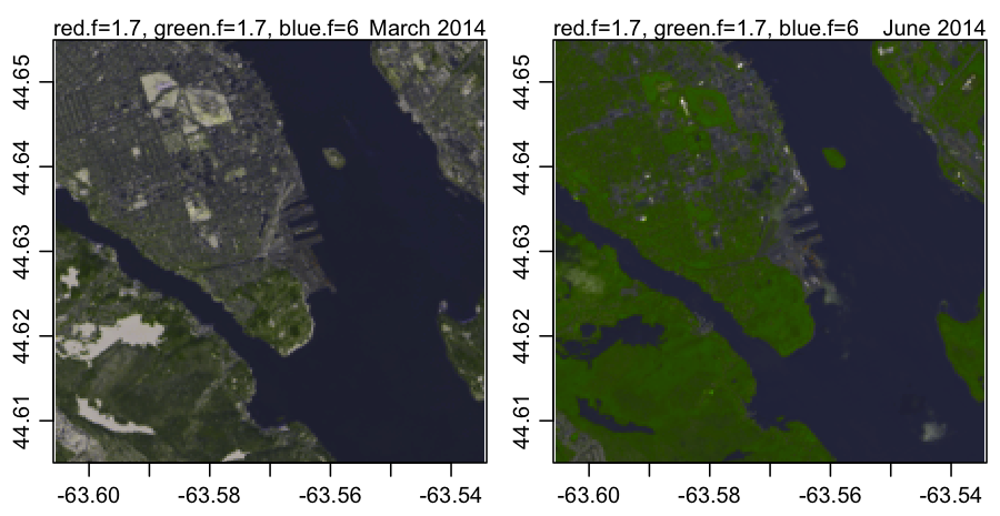
**Case 3.**

Decrease red and increase blue, which neutralize the winter hue (especially of
the snow-covered citadel) and of summer paved (especially Pier 21 and railway
funnel).  The asphalt regions (e.g. the dockyard, year-round) are now a neutral
gray.  A blue hue covers water in both seasons. The summertime greens are
rather bright, but this is what this tree-covered region looks like.

The lakes on the south side of the Northwest Arm are probably covered with
smooth and rather clean snow, and so it is agreeable that the colour is both
brighter there than on the citadel, which is, after all, a fort surrounded by a
steep hill.

Overall, I am quite satisfied by the neutrality of both the ice/snow and darker
asphalt/gravel regions.  The greens also look good, and close inspection of the
winter image will show greens in the parts of Halifax that have coniferous
trees.

The main remaining question is whether the coefficients will handle red
properly, because there are no prominent red items in this view.  My
experiments have shown that a neutralization of the gray/white regions can be
achieved with a variety of red-blue pairings, and so I would like to have
another test image that will help me to set that balance in a way that works
for both the green-gray domain of Halifax and some other domain.  If any reader
wants to help with that, please contact me directly (since I do not have
comments turned on for this blog).

```{r eval=FALSE}
demo(1.7, 1.7, 6, "2016-02-20-landsat-3.png")
```
![center](https://dankelley.github.io/figs/2016-02-20-landsat-3.png) 

# Conclusions

These tests suggest that the values `red.f=1.7`, `green.f=1.7` and `blue.f=6`
may be more reasonable as defaults than the present values of 2, 2, and 5,
respectively.  I will wait a week for any personal advice from colleagues, and
consider switching the defaults after that time.

# References and resources

1. [issue report on landsat hue](https://github.com/dankelley/oce/issues/874)

2. Jekyll source code for this blog entry: [2016-02-20-landsat-hue.Rmd](https://raw.github.com/dankelley/dankelley.github.io/master/assets/2016-02-20-landsat-hue.Rmd)